Skip links

From Decision Exhaust to Intelligent Enterprise Architecture thru Ontology & Palantir

In the first article, I introduced the idea that most enterprises stop at automation, but very few become truly intelligent machines.

Over the past few decades, enterprises have invested heavily in ERP modernization, cloud data platforms, AI capabilities, BI dashboards etc. Yet still during peak operational periods, most organizations still rely on spreadsheets, escalation emails, war-room meetings, and manual overrides.

Most companies automate tasks. Very few redesign how decisions are made, governed, executed, explained, and learned from.

In this article, I would like to explore this further on what does it actually take to implement an Intelligent Enterprise architecture. To illustrate this, I would like to use Palantir as an example. This also helps clarify what #palantir does since most people still think palantir just as yet another data or AI platform. In reality, it is a system that models how a business operates so decisions can be made, executed, and learned from end-to-end.

How do data, decisions, workflows, GenAI, and enterprise integrations come together into a single Palantir system?

The Intelligent Enterprise

To keep this grounded, we will continue using the same use case:

A retailer, Planning and Allocating a Black Relaxed Hoodie across 100 stores.

The Use Case

  • Retailer: OmniRetailCo
  • Product: Black Relaxed Hoodie
  • Stores: 100
  • Distribution Center: Dallas
  • DC Planning Week: Week 39

Initial demand signals for few stores for illustration:

StoreForecast (P50)Forecast (P90)
Dallas120150
Austin110135

Total demand across the store network ≈ 12,000 units

But the Dallas distribution center can only process: 8,000 units

This mismatch between demand and capacity is what we will architecture and it will hopefully pave the path to solving the decision exhaust problem within Enterprises.

1. Define the Operational Language (Ontology)

The foundation of the #Palantir system is a shared operational language. In #Palantir Foundry, this is implemented using the Ontology, where business entities are modeled as object types backed by datasets.

Core objects:

  • Product
  • Store
  • Distribution Center
  • Forecast
  • Allocation
  • Recommendation
  • Decision
  • Outcome
  • Policy Rule
  • Scenario
  • Decision Exhaust

Example Product dataset:

product_idskuproduct_namecostretail_price
P100BRH-01Black Relaxed Hoodie4060

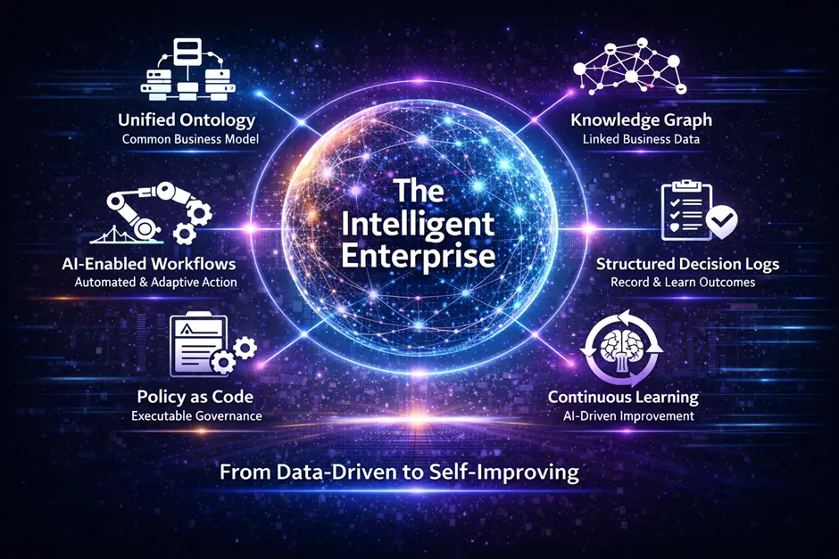
These objects form the digital twin of the enterprise — a living model of business operations that applications, workflows, and AI systems operate on.

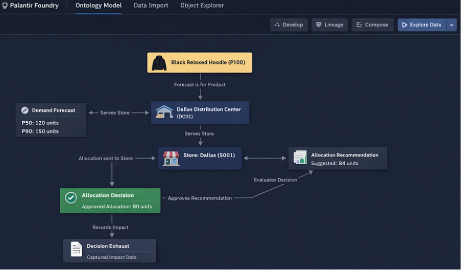
2. Define Relationships in Business Language

Relationships between ontology objects are defined using link types, which are expressed in plain business language.

Examples:

  • Forecast is for Products
  • Forecast is for Stores
  • Stores is served by Distribution Center
  • Distribution Center fulfills Stores
  • Recommendation suggests allocation for Stores
  • Decision approves Recommendation
  • Decision applies Policy Rule
  • Outcome evaluates Decision

These relationships are not just structural. They are semantic and readable. In cases where relationships require context, object-backed links are used. This allows relationships themselves to carry business operational meaning.

ontology model chart

3.  Build Data Pipelines, Lineage, and Context

All business operational data flows through pipelines built in #palantir Foundry using:

  • Pipeline Builder
  • Code Repositories (Python / Spark / SQL)

Typical data sources:

  • POS transactions
  • Inventory snapshots
  • Shipments
  • Promotions
  • Capacity data
  • Vendor inputs

Pipelines transform these into structured datasets for demand planning, forecasting and optimization.

Every dataset is fully traceable through Data Lineage:

  • Upstream source
  • Transformation logic
  • Downstream consumers

AI is embedded directly in pipelines to process unstructured inputs:

  • Extract promotion details from documents
  • Classify vendor communications
  • Summarize operational notes
  • Normalize free-text inputs into structured signals

This ensures the operational graph can tap into organizational intelligence in the form of both structured and unstructured data.

4. Demand Planning,  Forecast Generation and Model Lifecycle

Forecasts (P50, P90) are generated using machine learning models built and managed in #panatir Foundry.

Example:

Storeforecast_p50forecast_p90
Dallas120150
Austin110135

Models are:

  • Versioned
  • Monitored
  • Retrained
  • Deployed

Using AIP Analyst, planners can interact with forecasts using natural language where AI can interpret and reason:

  • Explain forecast changes
  • Identify drivers of demand
  • Compare forecast accuracy

AI acts as a natural language interface over model outputs and lineage.

5. Operational Applications

Planners interact with the system through Operational Applications (Workshop).

A planner viewing a product sees:

  • Demand signals
  • Inventory
  • Allocations
  • DC capacity
  • Risks
  • Scenarios

Different applications exist for different personas – Demand Planner, Allocation Analyst, Store Manager, Executives etc.

Inside applications, AI acts as a copilot:

  • Explain operational issues
  • Summarize risk
  • Highlight anomalies
  • Answer business questions
6.  Generate Allocation Recommendations

At this stage, the system is solving a constrained business decision problem using the operational graph defined in the ontology.

The objective is not just to predict demand, but to: “Maximize margin under real-world constraints”

The system brings together all relevant signals into a single decision context:

  • Demand signals (Forecast P50 / P90 etc.)
  • Supply constraints (DC capacity = 8,000)
  • Inventory availability
  • Store performance (sales velocity, conversion rates)
  • Financials (margin per unit = $20)
  • Policy rules

The system translates this into a constrained optimization problem.

a) Starting with unconstrained demand:

  • Dallas demand = 120
  • Austin demand = 110
  • Total demand ≈ 12,000 units

If there were no constraints, the system would allocate to meet full demand.

b) Apply capacity constraint at DC

  • Total available capacity = 8,000 units
  • Shortfall = 4,000 units

This forces the system to decide where to allocate limited supply.

c) Score each store

Each store is assigned a priority score based on:

  • Demand level
  • Sales velocity
  • Margin contribution
  • Historical performance

Example:

StoreDemandVelocityMarginScore
Dallas120HighHigh0.92
Austin110MediumHigh0.88

d) Allocate proportionally with constraints

The system could evenly distributes inventory using a weighted allocation approach or using some sophisticated constrained optimization approach:

  • Higher score → higher share of constrained supply
  • Ensures total allocation ≤ 8,000
  • Ensures fairness / policy limits are respected
storeCurrentrecommended
Dallas8084
Austin8082

e) Apply policy adjustments

Policies further refine the output:

  • Avoid extreme deviations across stores
  • Cap allocation shifts
  • Enforce minimum thresholds

These are also stored as Allocation Recommendation Ontology objects.

AI explains recommendations:

  • Why allocation changed?
  • What constraints influenced it?
  • Summarize tradeoffs?

Example reasoning:

  • Dallas has higher forecast demand (120 units)
  • Sales velocity is above average (+12%)
  • Higher margin contribution relative to other stores
  • Allocation reduced from unconstrained demand due to DC capacity limit
  • Redistribution applied across all stores

Because relationships are defined in business language in the ontology, the system can express this in plain English:

“Dallas store received a higher allocation because it is linked to the product with stronger demand and higher sales velocity. However, the allocation was limited due to the Dallas Distribution Center capacity constraint, which required redistribution across all stores”

f. Tradeoffs Are Explicit

The system also evaluates what it could not do due to policies making the decision transparent,

  • Increasing Dallas further would reduce allocation to other stores
  • Total allocation must remain within 8,000 units

g. AI as the Reasoning Layer

GenAI is embedded at this stage to:

  • Explain why recommendations changed
  • Summarize constraints and tradeoffs
  • Simulate alternative scenarios
  • Allow planners to ask questions in natural language

What happens if we prioritize top-performing stores only and the system can recompute and explain instantly and help enable what if analysis and simulation

7.  Evaluate Recommendations Against Policies

At this stage, the system has produced a proposed allocation with full reasoning. But recommendations cannot execute blindly. They must be evaluated against explicit business policies. Policies are modeled as first-class objects in the ontology and linked to decisions.

Example policies:

PolicyConditionAction
Auto-approve small changesΔ ≤5%Approve
Capacity ConstraintTotal Allocation > 8,000Rebalance
High margin riskLost margin $50KEscalate

The system evaluates each recommendation by computing:

  • Delta from current allocation
  • Aggregate allocation across all stores
  • Projected margin impact
  • Constraint violations

Dallas recommendation:

  • Current allocation = 80
  • Recommended = 84
  • Delta = +5% → qualifies for auto-approval

Also perform global check:

  • Total recommended allocation = 9,000
  • Capacity = 8,000 → constraint violated

The system does not reject the recommendation outright. It resolves the conflict by:

  • rebalancing allocations across stores
  • prioritizing higher scoring stores
  • maintaining policy constraints

This produces a policy-compliant recommendation set. AI explains policy outcomes in plain language:

The recommendation was adjusted because total allocation exceeded the Dallas DC capacity. The system redistributed units across stores while maintaining priority for high-performing locations.

It can also answer: Which policy caused this change? What would happen if we relaxed the threshold?

8. Workflow Execution, Decisions, and ERP Integration (MCP)

At this point, the system moves from reasoning → action orchestration.

A workflow is triggered automatically when:

  • New recommendations are generated
  • Policy evaluation is complete

The workflow engine performs:

  • Classify the decision (auto-approve -> require approval -> escalate)
  • Route the decision (Planner -> Director, MP&A -> VP, MP&A)
  • Automated execution

Track state transitions (pending -> approved/rejected -> executed)

Human-in-the-Loop (When Needed):

Planners can review recommendations, see reasoning and tradeoffs, override decisions, leave comments etc. All actions are captured in the system.

Once approved, the decision will be executed in operational systems such as ERP.

Instead of tightly coupled APIs, the system uses MCP (Model Context Protocol) to execute actions.

  1. Decision is approved in Foundry
  2. Action Type is triggered (e.g., “Update Allocation”)
  3. MCP generates a structured tool call
  4. ERP system consumes the action
  5. Execution status is returned
  6. Status is written back to the ontology closing the look and enabling bi-directional integration

{

“action”: “update_allocation”,

“store_id”: “Dallas”,

“product_id”: “P100”,

“approved_units”: 80

}

9. Measure Outcomes, Capture Decision Exhaust, and Drive Learning

At this point, the system has already:

  • Generated recommendations
  • Applied policies
  • Executed workflow
  • Pushed decisions to ERP via MCP

Now the question is: Did the decision actually work and is this the best decision the team could have taken? This is where true intelligence actually begins. Test -> Learn -> Refine.

Once allocations are executed, real-world business outcomes flow back into the system.

StoreApproved AllocationObserved Sales
Dallas8080
Austin8078

Observed sales are constrained by supply, not pure demand. The system reconstructs demand using:

True Demand = max(Forecast, Observed Sales)

StoreForecastSalesTrue Demand
Dallas12080120
Austin11078110

This step separates from “What happened?” to “What could have happened?” Now the system calculates the consequence of constraints.

Inputs:

  • Retail price = $60
  • Cost = $40
  • Margin = $20

Example:

StoreTrue DemandAllocationLost UnitsLost Margin
Dallas1208040800
Austin1108030600

At scale:

  • Total demand = 12,000
  • Allocation = 8,000
  • Lost units = 4,000
  • Lost margin = $80,000

This happens to be the financial consequence of the decision.

10. Capture Decision Exhaust as a Complete System Record

Now the system captured everything that led to this outcome. It is a fully connected dataset that preserves the entire lifecycle of a decision.

Comprehensive Decision Exhaust Model

decision_exhaust:

decision_id: “Unique identifier for this decision”

product: “Product being planned (e.g., Black Relaxed Hoodie)”

store: “Store where the decision was applied”

planning_week: “Week of execution”

demand_signal:

forecast_p50: “Baseline expected demand”

forecast_p90: “Upside demand potential”

recommendation:

suggested_allocation: “System recommended units”

confidence_level: “Confidence in recommendation (0–1 scale)”

key_drivers:

– “Primary factors influencing the recommendation (e.g., demand, velocity)”

tradeoffs_considered:

– “What the system had to balance or sacrifice”

final_decision:

approved_allocation: “Final units approved for execution”

change_from_recommendation: “Difference from suggested allocation”

policy_applied: “Policy that influenced the decision”

constraint:

type: “Type of constraint (e.g., capacity, policy, manual override)”

impact_level: “Severity of constraint impact (low / medium / high)”

approval_details:

approval_flow:

– “Planner”

– “Director”

– “VP”

overridden: “Was the recommendation overridden? (true/false)”

override_reason: “Reason for manual override (if applicable)”

execution:

execution_status: “Success / Failed / Pending”

execution_time: “Timestamp when action was executed in ERP”

outcome:

actual_sales: “Units sold”

estimated_true_demand: “Demand including unmet demand”

unmet_demand_units: “Units that could not be fulfilled”

lost_margin: “Revenue impact due to unmet demand”

context:

scenario: “Scenario under which the decision was made (if applicable)”

Example:

StoreForecastRecommendedApprovedSalesTrue DemandLost MarginPolicyConstraint
Dallas120848080120800CapacityDC Limit

Because the system captures decision + context + outcome together, it can now answer:

  • Which constraints consistently reduce margin?
  • Which stores are systematically under-allocated?
  • Which policies are too conservative?
  • Where do overrides happen most often?
  • Which decisions delivered the highest ROI?

AI as the Reasoning Layer Over Decision Exhaust

  • Operating over structured decision history.
  • Explain why decisions failed
  • Summarize weekly performance
  • Identify recurring patterns
  • Recommend policy changes

  • Suggest capacity investments

Example:

Dallas stores consistently lose margin due to DC capacity constraints. Increasing capacity by 10% would reduce lost margin by approximately $12,000 per week.

It can also answer:

  • What are the top 5 constraints impacting margin?
  • Which decisions required overrides most often?
  • What policy changes would improve outcomes?
11. Close the Learning Loop

Now the system feeds this intelligence back into itself for continuous learning and recommendation

  • Forecast models – Learn from true demand (not constrained sales)
  • Allocation logic – Adjusts prioritization based on impact
  • Policies – Evolve based on outcomes
  • Capacity planning – Becomes data-driven

Now, The system now operates as a continuous loop:

Signal → Recommendation → Policy → Action → Outcome → Decision Exhaust → Learning

  1. “Most systems remember data”,
  2. “Very few systems remember decisions”,
  3. “Fewer still understand their consequences”

An Intelligent Enterprise does all three!

This website uses cookies to improve your web experience.
Home
Account
Cart
Search